# Audio Programming > "Music is a secret calculation done by the soul unwaware that it is counting", W. Leibniz. This part of the course is all about generating audio by writing code. The audio might be music, it might be sound design, it might be transformations of existing sounds or generative production of genuinely new sounds. Whatever it is, it will be partially defined by the creation of an algorithm expressed as code. We'll also be biased toward creative expression through code, for the sheer fun of it. > It isn't a course about DSP (Digital Signal Processing); to learn more about that fascinating field take a look at [Julius Smith's online resources](https://ccrma.stanford.edu/~jos/) or any DSP course in Electrical Engineering, for example. But we will encounter some DSP principles and examples along the way. Similarly, it isn't about music or sound design as such, though we may also visit some musical concepts and a bit of computer music history as we go. Today we spend half of our lives listening to computer mediated sound. Research questions include how to better control that sound in intuitive or interesting ways; how to generate sound that more closely approximates the real; or alternatively to generate sounds that we have never heard before; how to distribute sound more effectively (in physical or virtual spaces); how to process it more efficiently; how to analyze and reconstruct sound intelligently; and so on. ## Digital representation of sound Sound recording/playback technology requires a mechanism to transform the ephemeral undulations of sound pressure (what we can hear) into a persistent record, and another mechanism to the transcribe this record back into waves of sound pressure. In the phonograph (below), introduced in 1877, vibrations in the air are amplified by the horn to vibrate a stylus, etching patterns into a rotating cylinder. The same mechanism can be used for recording and playback.  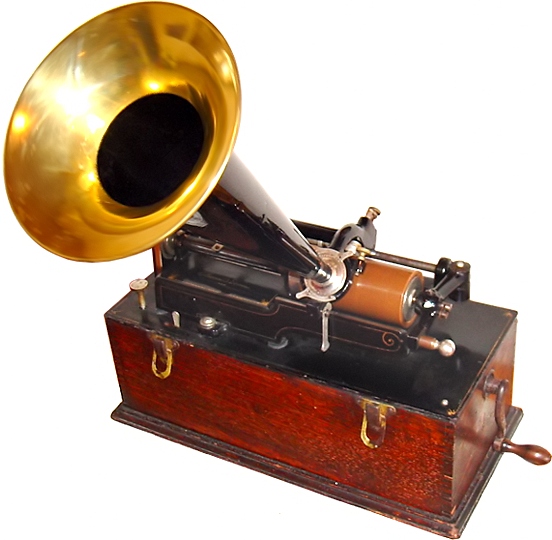The modern record player adds an electronic amplifier to drive the movements of a loudspeaker cone, but otherwise follow the same princple. Here are vinyl record grooves under an electron microscope:  These grooves are smooth and continuous, since records are an **analog** representation of sound, which is theoretically ideal. Unfortunately it is susceptible to noise and gradual degradation. The **digital** representation of sound on the other hand is completely discrete:  At the simplest level, sounds are represented digitally as **a discrete sequence of (binary encoded) numbers**, representing a time series of quantized amplitude values that relate to the variations of compression an expansion in the air pressure waves we hear as sound. It is bound by the sampilng theorem and other aspects of [information theory](http://en.wikipedia.org/wiki/Information_theory), just like any other digital representation. > This has important implications in the field of data compression. An MP3 file encodes the content of a sound file by removing parts of the sound that are less significant to perception, requiring much less memory to represent a sound. **Lossless** codecs (such as FLAC) compress sound without audible reduction in quality at all. However, to play back a compressed file we must first uncompress it again, returning it to a simple series of discrete amplitude values. Computers are fundamentally discrete. This applies in two ways: 1. All values in memory are represented using **discrete encoding** (ultimately binary). Binary representations of number impose limits due to finite memory. Integers are limited to a certain range (for example, 8-bit integers (***char***) can represent whole numbers between 0 and 255 inclusive, or -128 and 127 inclusive in the signed variant), and floating point numbers are limited to a certain resolution, unable to represent small differences between very large numbers. Complex data is represented by composition of smaller elements: for example an animation is made of several frames, each frame of several pixels, each pixel of several colors, represented by number. The number of colors, pixels and frames is also discrete and limited by available memory. 2. Computation proceeds in **discrete steps**, moving from one instruction to the next. Although this occurs extremely fast (millions of steps per second in current hardware), it remains discrete. The entire logic of computation is built upon a discrete series of instruction flow. Thus although we can represent continuous *functions* in the computer (e.g. by name), we cannot accurately represent continuous signals they produce, as they would a) require infinite memory or b) require infinitely fast computation to produce each infinitessimal value in sequence. Is this a problem? Instead we can **sample** a function so rapidly that we produce a series of values that are perceptually continuous. This is exactly how digital audio signals work. Digitized audio a discrete-time, discrete-level signal of a previous electrical signal. Samples are quantized to a specific bit depth and encoded in series at a specific rate.  How fast is fast enough? If the function changes continuously but only very slowly, only a few samples per second are enough to reconstruct a function's curve. You do not need to look at the sun every millisecond to see how it moves; checking once per minute would be more than enough. But if we didn't check fast enough, we might miss important information. If we checked the sun's position once every 26 hours, we might not be able to precisely understand the repetition of its movement. ### Frequency An event that occurs repeatedly, like the sun rising and setting, can be described in terms of its repetition period, or cyclic frequency (the one is the inverse of the other). period = 1 / frequency frequency = 1 / period In units: seconds = 1 / Hertz Hertz = 1 / seconds - The sun's traversal of the Earth's sky has a period of 1 day (approximately 93,600 seconds), which is 0.00001068376 cycles per second (Hz). Long periods imply low frequencies. - The heart beats around 60-100 times a minute (bpm). This also happens to be the typical range of frequencies for musical meter. 60bpm is a frequency of 1 cycle per second (1Hz). - The lowest frequencies that we perceive as tones begin at around 20 cycles per second (20Hz). That is, every 0.05 seconds (50 milliseconds). The region between rhythm and tone, around 8-20Hz is very interesting: this is where most vibrato modulation is found. - The persistence of vision effect which allows image sequences to appear as continuous motion begins at around 10-20 frames per second (Hz), depending on content. Cinema traditionally used 24 or 30 frames per second. Rapid movements in modern gaming may demand frame rates of up to 60Hz or more. - Human singing ranges over fundamental frequencies of about 80Hz to about 1100Hz. - What we perceive as timbre, or sound color, consists mostly of frequencies above 100Hz well into the thousands of Hz (kHz). For example, we distinguish between different vowel sounds according to proportions of frequencies (called formants) in the range of 240 to 2500 Hz. A high hat cymbal is largely made of a complexity of much higher frequencies. - Human auditory perception begins to trail off above 10000 - 20000 Hz (10 - 20kHz), depending greatly on age. Sounds above these frequencies are audible to many other species. A high frequency of 20kHz implies a cyclic duration of just 0.00005 seconds. High frequencies imply short durations. The fact that the whole gamut of musical phenomena, from an entire composition of movements, to meter and rhythm, to pitch and finally sound color can be described by a single continuum of time has been noted by composers such as Charles Ives, Henry Cowell, Iannis Xenakis and Karlheinz Stockhausen. Stockhausen 1972 Oxford lectures (YouTube) ### Sampling Theorem So how fast is fast enough? How often must you check the sun's position to know its period? Once sample per day would not be enough: the sun would appear to not be moving at all. One sample every 23 hours would only see a complete cycle every 24 days, and would make the sun appear to be slowly moving backwards! The incorrect reperesentation of frequency due to insufficient sampling is called **Aliasing**.  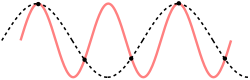In fact the minimum period necessary to correctly measure the sun's frequency is 12 hours: enough to capture both night and day (or sunrise and sunset). Sampling more frequently would more accurately capture the actual curve traversed, but 12 hours is enough to capture the frequency. The (Nyquist-Shannon) sampling theorem states that a sampling of a certain frequency R is able to represent frequencies of up to one half of R. Frequencies above one half of R may be represented incorrectly due to aliasing. A classic example of aliasing is the "wagon wheel effect". Standard audio CDs are encoded at a sampling rate of 44100Hz, which means a frequency of 44100 samples per second. That implies they can represent frequencies of up to 22050Hz, close to the limit of human perception. The bit depth of CD audio is 16 bits. DVD audio uses a higher sampling rate of 48000Hz. Many audio devices support up to 192kHz and 24 bits. (When processing audio in the CPU however, we generally use 32 or 64 bit representations.) A more detailed explanation with diagrams [in the dspguide here](http://www.dspguide.com/ch3/2.htm) ### Bit depth The quantization bit depth of the representation determines the signal to noise ratio (SNR), or dynamic range. Every bit of resolution gives about 6dB of dynamic range, so a 24 bit audio representation has 144dB. The [decibel](http://en.wikipedia.org/wiki/Decibel) (dB) is a logarithmic unit to represent a ratio between to quantities of intensity. "The number of decibels is ten times the logarithm to base 10 of the ratio of the two power quantities." (IEEE Standard 100 Dictionary of IEEE Standards Terms). A change by a factor of 10 is a 10dB change, and a change by a factor of 2 is about a 3dB change. Decibels are frequently used in two ways in audio: 1. To represent the acoustic power of a signal, relative to a standard measure approximating the minimum theshold of perception. The loudness of different sound-making devices can be measured in decibels, which will typically be positive (louder than the reference threshold). 2. To represent the signal-to-noise ratio of a digital representation. In this case signals are measured in reference to the *maximum* power signal (amplitude value of +/- 1), and thus are typically negative. OdB indicates full power. Positive dB indicates signals above the representation range, which will be clipped, and negative dB indicates quieter signals. The range between full power and the smallest representable (nonzero) signal specificies the signal-to-noise ratio of a representation. The human ear can discriminate around 120dB of dynamic range, though this is frequency dependent. A 16 bit depth (standard CDs) provides around 120dB. However when operating and transforming audio greater headroom is needed. 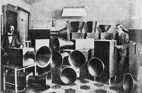## The Great Computer Music Problem Many early electronic and computer music composers were attracted to the medium for the apparently unlimited range of possible timbres it could produce. One hundred years ago the avant-garde of Western music were experimenting by broadening the sonic palette of Western music, to the point that Italian Futurist composer Luigi Russolo conceived of "noise music" concerts, new noise instruments ("Intonarumori") and the manifesto "The Art of Noises"; in part responding to the industrial revolution, in part continuing the trend of breaking down classical music principles, and no doubt in part also the sheer fun of it...  In addition to the potential to find [the new sound](http://www.youtube.com/watch?v=pQLlR4pvhyg), the computer was also attractive to composers as a precise, accurate and moreover obedient performer. Never before could a composer realize such control over every tiny detail of a composition: the computer will perfectly reproduce the commands issued to it. Unfortunately, although the space of possible sounds in just one second of CD-quality audio is practically infinite, the vast majority of them are uninteresting. For example, as we heard already, simply selecting the samples randomly results in psychologically indistinguishable white noise. Specifying each sample manually would be beyond tedious. So, with all the infinite possibilities of sounds available, how *should* one navigate and control the interesting ones? (This is precisely the problem posed in Homework 1: how to design an interesting function to map from discrete time to an interesting sequence of audio samples.) What are the salient general features that we perceive in sound, how can they be generated algorithmically, with what kinds of meaningful control? ### Music-III One of the most influential solutions to this problem was developed by Max Mathews at Bell Labs in the late 1950's, in his **Music-N** series of computer music languages. The influence of his work lives on today both in name (Max in [Max/MSP](http://en.wikipedia.org/wiki/Max_(software)) refers to Max Mathews) and in design (the [CSound](http://en.wikipedia.org/wiki/Csound) language in particular directly inherits the Music-N design). - [Mathews, M. An Acoustic Compiler for Music and Psychological Stimuli](http://ia601505.us.archive.org/7/items/bstj40-3-677/bstj40-3-677.pdf) Mathews' approach exemplifies the "divide and conquer" principle, with inspiration from the Western music tradition, but also a deep concern (that continued throughout his life) with the psychology of listening: what sounds we respond to, and why. In his schema, a computer music composition is composed of: - **Orchestra**: - Several **instrument** definitions. - Defined in terms of several **unit generator** types (see below), - including configuration parameters, - and the connections between the unit generators. - **Score**: - Some global configuration - Definition of shared, static (timeless) features - Many **note** event data, referring to the orchestra instruments, - including configuration parameters. Matthews was aware that we perceive time in combinations both discrete events and continuous streams; abstracted into his "note" and "instrument" components. The "score" is able to reflect the fact that we perceive multiple streams simultaneously. 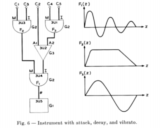#### Unit Generators He also noted that streams are mostly formed from approximately periodic signals, whose most important properties are period (frequency), duration, amplitude and wave shape (timbre), with certain exceptions (such as noise). Furthermore he noted that we are sensitive to modulations of these parameters: vibrato, tremelo, attack (rise) and decay characteristics. To provide these basic characteristics, without overly constraining the artist, he conceived the highly influential **unit generator** concept.  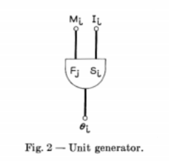Each unit generator type produces a stream of samples according to an underlying algorithm (such as a sine wave) and input parameters. Unit generators (or simply "ugens") can be combined together, by mapping the output of one ugen to an input parameter of another, to create more complex sound generators, and ultimately, define the instruments of an orchestra. The combination of unit generators is called a *directed acyclic **graph***, since data flows in one direction and feedback loops are not permitted.  Some example unit generators include: - **Adder**. The output of this ugen is simply the addition of the inputs. In Max/MSP this is [+~]. - **Random generator**. Returns a stream of random numbers. In Max/MSP this is called [noise~]. - **Triangle ramp**. A simple rising signal that wraps in the range [0, 1). In Max/MSP this is called [phasor]. - In Music-II this is not a bandlimited triangle, and may sound harsh or incorrect at high frequencies. - **Wavetable playback**. For the sake of simplicity and efficiency, Music-III also featured the ability to generate **wavetables**, basic wave functions stored in memory that unit generators can refer to. The most commonly used unit generator simply reads from the wavetable according to the input frequency (or rate), looping at the boundaries to create an arbitary periodic waveform. In Max/MSP this could be [cycle~] or [groove~]. - In Music-III this does not appear to use interpolation, and thus may suffer aliasing artifacts. - **Acoustic output**. Any input to this ugen is mixed to the global acoustic output. This represents the *root* of the ugen graph. In Max/MSP this is called [dac~].  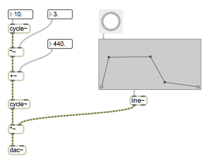*Here's what the above instrument looks like (more or less) in Max/MSP.* Modern computer music software may have hundreds of different unit generators. Max, PD, CSound and SuperCollider are particularly plentiful. #### Acoustic compiler Music-III is a **compiler**, that is, a program that receives code in some form, and produces a program as output. (More generally, programs that create programs are called *metaprograms*). Given **orchestra** specification data, the Music-III compiler produces programs for each of the **instruments**. A separate program, called the **sequencer**, receives score data, and for each note, the sequencer "plays" the corresponding instrument program, with the note parameters to specify frequency, volume, duration etc. The outputs of each note program are mixed into an output stream, which is finally converted into sound. In summary: 1. Compile instrument definitions into programs. 2. Sequence note events to invoke instruments and write results into output. The benefits of his approach included both flexibility (a vast diversity of instruments, orchestrae, scores can be produced), efficiency (at $100 per minute!), and suitability to producing interesting sounds. In Music-III a unit generator graph, or *instrument*, as above would be specified by a series of macro instructions: first to define the unit generators (type, parameters, output connections), and to specify which note parameters map to which unit generator inputs. Although the syntax is very different (and we no longer need to punch holes in card!), the same principles are clearly visible in modern computer music languages, such as the SynthDef construct in [SuperCollider](http://en.wikipedia.org/wiki/SuperCollider): ``` ( SynthDef(\example, { Out.ar(0, SinOsc.ar(rrand(400, 800), 0, 0.2) * Line.kr(1, 0, 1, doneAction: 2) ) }).play; ) ``` #### Sequencer After the orchestra is compiled, the score is input to a sequencer routine, to drive creation of the final composition. Score events include: - Specifying the generation of *wavetables*. - Specifying the time scale / tempo. - Specify note events (with parameters including instrument ID, duration, and other instrument-specific controls). - Punctuation: - rests, - synchronization points, - end of the work. Note that the structure of a composition (orchestra, score) is strict but includes variable components. It could be modeled as a data structure, or as a grammar for a domain-specific language (such as CSound). With modern languages we can overcome many of the limitations in the 1950's programming environment, allowing us to create a much richer and friendlier acoustic compiler and sequencer... > Is this the only way to structure a composition? Is it the only/best solution to the great computer music problem? What cannot be expressed in this form? What alternatives could be considered? ### The Software Development Process [We found that](https://github.com/grrrwaaa/gct633/blob/master/classfiles/sep17.lua) we could define unit generators as **constructor** functions that return sample-making functions. The assumption is that the input arguments to a unit generator constructor are also sample-making functions: ``` -- construct a unit generator f -- inputs a and b are sample-making functions: function make_adder(a, b) -- the unit generator function created: return function() -- compute the next values of the two sample-making inputs -- then return their sum: return a() + b() end end ``` As is often the case in programming, this is not the only way to do it. It might not be the most efficient; it might not scale well; but it happens to be a fairly simple one to write. This is an important heuristic in [agile software development](http://agilemanifesto.org/): 1. **Make it work** (i.e. satisfy the minimum requirement to be able to use it) 2. **Make it right** (i.e. eliminate errors, handle special cases, begin to generalize) 3. **Make it fast** (i.e. avoid waste) > What this means is always solve problem (1) first, before moving on to (2) and later (3), if needed. This far from the only principle of [Agile development](http://en.wikipedia.org/wiki/Agile_software_development), but it does reflect the importance of fast turnaround and evaluation for *informed* development. Although it may not be obvious, our current plan fails on point 1. After playing around with it for a while, you might find a problem in the following case. The result should be a louder 1000Hz signal, but what we get instead is a 2000Hz signal. *Why?* ``` -- create an instrument that adds two 1000Hz sinewaves at 50% amplitude: local u1 = make_sine(const(1000), const(0.5)) local u2 = make_adder(u1, u1) ``` One value of developing in the Agile style is that this problem is encountered early, before a huge infrastructure has been created. This problem requires a major change to the system, which would be costly (or boring) if encountered at a later stage. Similarly, we can build the sequencer component in the simplest and most naive way first, to make sure it works; then by using it we may find what special cases it does not handle, what additional features may be desirable, and whether the performance needs to be improved. The sequencer's basic requirements: - Support a **score** (list) of note events. - Both score, and note events, could be modeled as Lua tables. - Each note refers to an instrument - Each note may have other parameters - The **sequencer** function should mix the score's notes into the output - This means iterating through the list of notes, and playing those that should be active at any time. - This means invoking the instrument somehow - Including variation according to the note parameters - The outputs of concurrently playing notes should be added together. ---- ## Lazy Programming Many programmers are lazy, and many programmers like laziness. Laziness is one of the great motivators for innovation. For example, abstraction appeals to our desire to be lazy, as it makes future revisions easier. [Lazy evaluation](http://en.wikipedia.org/wiki/Lazy_evaluation) is a technique of software design in which values are computed as late as possible: only when they are needed. Lazy evaluation also implies not repeating the same computation twice (sharing results instead). It is sometimes referred to as **call by need**. Rather than computing each intermediate value on the way to a result, we can instead collect a description of the steps required, and only at the last moment actually execute them. This is also known as **deferred evaluation**. If we discover as we go that some of these steps were not necessary, we can remove them before executing. It also means that we can refer to values before they have been computed (these are called **futures**). In addition to improving performance (reducing waste), lazy evaluation can be used to represent potentially infinite data structures (you can add more on the end when you need them), and to define control flow in abstract rather than primitive forms. ### Lazy reaction Consider the orchestra/score. The score contains an ordered list of pairs, mapping discrete times to note objects. At each one of these times, the running *state* (the active set of notes) changes, but between these times it does not change. Between these times the (relatively) continuous behaviors of the notes generate changing sound, but the behaviors themselves do not change. Conal Elliot described a "reactive" appraoch to programming in a similar way: "Observed over time, a reactive behavior consists of a sequence of non-reactive phases, punctuated by events." [Elliot, C. Push-Pull Functional Reactive Programming ](http://conal.net/papers/push-pull-frp/push-pull-frp.pdf) ---- ## Excitation-resonance and other physical models It is widely and often commented that purely electronic sounds are too thin, shallow, artificial, cold, pure, etc. We should know that this criticism does not apply to computer-generated sound *in principle*, as we can reconstruct rich, deep, impure sounds during sample playback. The criticism really applies to the mathematical models that have been often been used to solve the computer music problem. One response to this has been to attempt to recreate nature in the computer, by running simulations of the physical (usually kinetic, mechanical) systems of musical instruments. In the computer music community it is often referred to as **physical modeling**. A "model" predicts the behavior of a physical system from an initial state and input forces. A "physical model" is one using systems drawn from physics, such as mass-spring-damper systems. [Julius Smith's online book of physical modeling](https://ccrma.stanford.edu/~jos/pasp/) Most acoustic physical models describe a process in which a source of energy (the "excitation") is transduced into the physical system, and then propagates as waves constrained by the system as a medium ("resonance"), some of which energy is transferred to pressure waves in the air ("sound") reaching our ears ("reception"). In fact most sounds that we hear in nature follow this form of excitation -> resonance. Several pheonomena are common: - After the excitation is removed, energy gradually dissipates away - The resonant objects (including the physical environment) emphasize certain frequencies over others (this is the "resonating" aspect), - High frequencies typically dissipate sooner than lower frequencies These are such fundamental aspects of natural sound that our psychoacoustic experience is hard-wired to them. Sustained sounds suggest a continuous input of energy. Crescendoes in nature are rare (wind, waves, approaching elephants). ### Vibrating strings Perhaps the simplest physical model is the vibrating string, such as found on a guitar or gayagum. The excitation is by plectrum or finger rubbing against and displacing the string (a short burst of randomized energy), or a bow continuously imparting random displacements (a longer, sustained input of noise). The resonance of the string is the vibrations it supports, which gradually decay as the energy dissipates into the instrument body. The body itself also resonates in a rich way, transducing energy to airborne sound. Because the string is constrained at each end, the only waveforms of vibration that can remain stable are proportional to integer divisions of the string length. This strongly constrains the sound produced, turning the rich spectrum of the noisy pluck into a more organized, decaying mixture of tones:  [Slow motion video of a bass string vibration](http://www.youtube.com/watch?v=XkSglALOueM) The simplest model of a vibrating string was presented by Karplus and Strong:  1. A noise burst (representing the pluck) is used as input added to a delay line. 2. The delay line length defines the fundamental tone of the string. 3. The feedback path includes a filter to emulate the way energy is gradually dissipated from the string (usually removing higher frequencies more quickly than lower ones). The gain of the filter must be less than 1 to avoid saturated feedback. --- ## Granular synthesis and microsounds Granular synthesis is a basic sound synthesis method that operates by creating sonic events (often called "grains") at the microsound time scale. > Microsound includes all sounds on the time scale shorter than musical notes, the sound object time scale, and longer than the sample time scale. Typically this is shorter than one tenth of a second and longer than ten milliseconds, including the audio frequency range (20 Hz to 20 kHz) and the infrasonic frequency range (below 20 Hz, rhythm). - [Microsound (Curtis Roads)](http://books.google.co.kr/books/about/Microsound.html) is the principal textbook Microsound was pioneered by physicist Denis Gabor and explored by composers Iannis Xenakis, [Curtis Roads](http://www.youtube.com/watch?v=0mQ8zRZOlrk), [Horacio Vaggione](http://www.youtube.com/watch?v=K-FjnKiDWQc), [Barry Truax](http://www.youtube.com/watch?v=X7FoPo-kyoM), [Trevor Wishart](http://www.youtube.com/watch?v=lekLl7o8yrc), and many more. Besides this, what is it useful for? - Impulse trains - Physical modeling of shaker-like instruments - Speech synthesis (e.g. FOF) - Wavelet analysis/resynthesis - Time/frequency resampling effects such as pitch-shifting and time-stretching - Separated processing of transients and stable waveforms, e.g. - Cricket chirps, frog croaks, etc. - Many other sonic textures of variable density, color, quality, and stochastic distributions Implementing a granular synthesis techinque involves two challenges: 1. **Specify the grain**: How to synthesize the individual samples of a grain (the *content*), how to specify the *duration*, what overall amplitude shape (the *envelope*) to apply, and how these can be parametrically controlled. 2. **Specify how grains are parameterized and laid out in time**: Whether to arrange grains at equal or unequal spacing, how densely they overlap, and so on; how to distribute parameter variations through the grains of a particular granular "cloud". Often clouds include stochastic distributions. ### Grain content Any sound source can be turned into a grain, by limiting the duration and choosing the envelope shape. It could be a mathematical synthesis technique, from a pure sine wave or noise source to a complex timbre. Or it could be a routine to select portions out of an existing waveform or input stream ("granulation"). With large populations of grains it can be very expensive to run complex routines for each grain. However as grain durations get shorter, there is less audible information stored in a grain and the exact synthesis algorithm becomes less important. Thus wavetable playback is often utilized. ### Grain envelope Similarly, envelopes can be either computed dynamically, or read from precalculated wavetable data. The shape of an envelope becomes increasingly important in determining the perceived sound as durations get shorter. Most envelopes begin and end at zero amplitude. Denis Gabor originally suggesed a Gaussian envelope shape, but today applications can make use of many mathematical and procedural envelope shapes. Often the envelope chosen is symmetric in time, rising from zero to peak at half-duration and falling back to zero; these shapes are frequently also used as **window** functions for signal analysis. The spectral properties of windows, represented by their Fourier transforms, are very significant in determining how well they suppress aliasing noise in the analysis (aliasing noise results from a time/space trade-off due to finite discretization). If we define "norm" as a ramp from 0 to 1 over the duration, and "snorm" as a ramp from -1 to 1 over the duration, we can define many classic window shapes: - Parabolic: 1 - snorm^2 - Cosine/Welch: sin(pi*norm), - Bartlett/Triangle: 2*min(norm, (1-norm)) - Gaussian: exp(-0.5 * (n*snorm)^2) - Blackmann: 0.42-0.5*(cos(2*pi*norm)) + 0.08*cos(4*pi*norm) - Hamming: 0.53836 - 0.46164*cos(2*pi*norm) - Hann: 0.5*(1-cos(pi*2*norm)) - Sinc/Lanczos: sin(pi*snorm)/(pi*snorm) - Nutall: 0.355768 - 0.487396*cos(2*pi*norm) + 0.144323*cos(4*pi*norm) - 0.012604*cos(6*pi*norm) - Blackman-Harris: 0.35875-0.48829*cos(2*pi*norm)+0.14128*cos(4*pi*norm)-0.01168*cos(6*pi*norm) - Blackman-Nutall: 0.3635819-0.4891775*cos(2*pi*norm)+0.1365995*cos(4*pi*norm)-0.0106411*cos(6*pi*norm) - FlatTop / Kaiser-Bessel: 0.22*(1-1.93*cos(2*pi*norm)+1.29*cos(4*pi*norm)-0.388*cos(6*pi*norm)+0.032*cos(8*pi*norm)) - Bessel: 0.402-0.498*cos(2*pi*norm)+0.098*cos(4*pi*norm)-0.001*cos(6*pi*norm) These an many other more complex window shapes are detailed [on the wikipedia page](http://en.wikipedia.org/wiki/Window_function), including time and frequency domain representations. 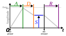Other envelope shapes are non-symmetric, and will impart stronger percussive or reverse effects to the sounds: - Inc: norm, Dec: 1-norm, Saw: snorm - Expodec: (1-norm)^n, Rexpodec: norm^n (and logarithmic versions for n<0) - Attack-release, attack-sustain-release, attack-decay-sustain-release and more complex linear, bezier or spline-segment shapes (some inspired by [note-envelopes common to synthesizers](http://en.wikipedia.org/wiki/Synthesizer#ADSR_envelope)) - Any symmetric window can be stretched by applying a non-symmetric transform to norm or snorm in advance.  In some cases an envelope is not needed at all, when the content can be arranged to have a natural intrinsic envelope shape. ### Grain distribution The principal method of combining grains into a cloud is called "overlap-add". A *scheduler* maintains a list of grains to play, working through the list of grains (sorted by grain onset time) and playing each grain in turn. Each grain adds its samples to the output buffer, accumulating onto (rather than replacing) the samples of any other previously played grains with which it overlaps. This is essentially the same as mixing multiple musical notes together, only with much shorter durations (and more accurately placed onset times). > In our software we already have sample-accurate overlap-add capability via audio.play() and audio.go()/audio.wait(). The great computer music problem appears again here: for populations of hundreds or thousands of grains, how to specify each grain's onset, duration, amplitude, spatial location and other parameters to create a meaningful result? Fortunately the situation for grains is more accessible than for individual samples. The spacing of grain onset times can be regular (*synchronous*) or irregular (*asynchronous*). Regular placement of grains can introduce another audible frequency effect. Holding the grain rate constant but varying the duration can achieve formant effects and simulate vocal sounds. With randomly distributed onset times however, density becomes a principal parameter. At longer time scales it can create [rhythmic](http://www.youtube.com/watch?v=uIeA2ct5Sew) or ["bouncing"]( http://www.youtube.com/watch?v=MA6ZXYIfLpA) effects. For granulation techniques, varying the start-point of the source waveform for each grain can be used to create time-stretching effects, or shifting the playback rate can be used to create pitch-shifting effects. Adding some random distribution to onset and duration can create a more organic, less metallic effect, but may weaken the strength of transients in the original. More generally, all parameters of a stream or cloud can be held constant, gradually shifted, randomly selected from a set, or distributed randomly around a center value as desired, to create many different complex shapes. Beyond this level, the task is to arrange the grains, streams and clouds together over space in time to construct a meaningful musical space. Changing the shapes of distributions over time was an important composition method of Iannis Xenakis. Beyond regular and random distributions, we could also explore the use of more generative algorithms such as Markov-chains, swarm dynamics and evolutionary algorithms. ---- ## Sounds as summations of cyclic rotations (Fourier) [A great interactive, visual explanation](http://toxicdump.org/stuff/FourierToy.swf) ---- ## Non-histories of computer music Delia Derbyshire (of Doctor Who fame): - [Delia Derbyshire circa 1963!](http://youtu.be/szE5D-dPs_Y) - [Delia Derbyshire etc. circa 1969!](http://youtu.be/K6pTdzt7BiI) ---- ## General Resources Online (free) texts: - [Julius Smith's online DSP books](https://ccrma.stanford.edu/~jos/) - [Miller Puckette's book](http://crca.ucsd.edu/~msp/techniques.htm) - [Steven Smith's DSP book](http://www.dspguide.com/pdfbook.htm) Non-free texts: - [Audio Programming Book](https://mitpress.mit.edu/books/audio-programming-book) - [Computer Music Tutorial](http://books.google.co.kr/books/about/The_Computer_Music_Tutorial.html?id=nZ-TetwzVcIC&redir_esc=y) - [Musimathics](http://www.musimathics.com/) - [Understanding DSP](http://www.amazon.com/Understanding-Digital-Processing-Edition-ebook/dp/B004DI7JIQ/ref=sr_1_1) - [Understanding Fourier (if you don't know math)](http://www.amazon.com/Who-Is-Fourier-Mathematical-Adventure/dp/0964350408/ref=sr_1_2?ie=UTF8&qid=1384225180&sr=8-2&keywords=who+is+fourier%3F) Forums - [KVR (a lot of DSP and plugin development stuff, since years ago!)](http://www.kvraudio.com/forum/) - [Create Digital Noise](http://createdigitalnoise.com/)